Auto neural networks vs. Manual Keras neural model
June 11, 2018
R modelling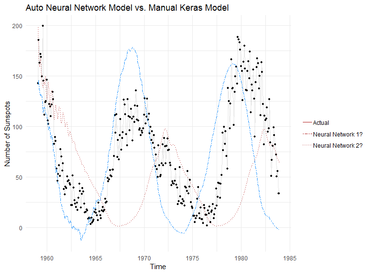
Several posts back I tested two packages for neural network time-series forecasting on the AirPassengers dataset.
I want to now test nnetar against a full neural network framework (Keras) and see how it fares.
Dataset
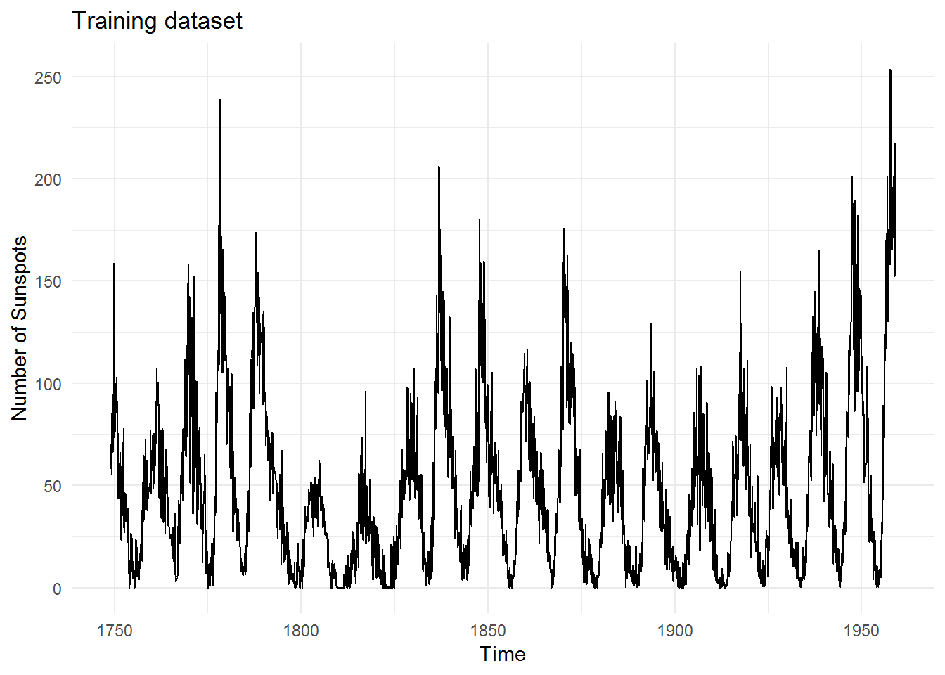
R contains a dataset called sunspots that is extremely long (starts from 1750s) and exhibits some nice seasonal patterns. This is the training data that we shall use for both models:
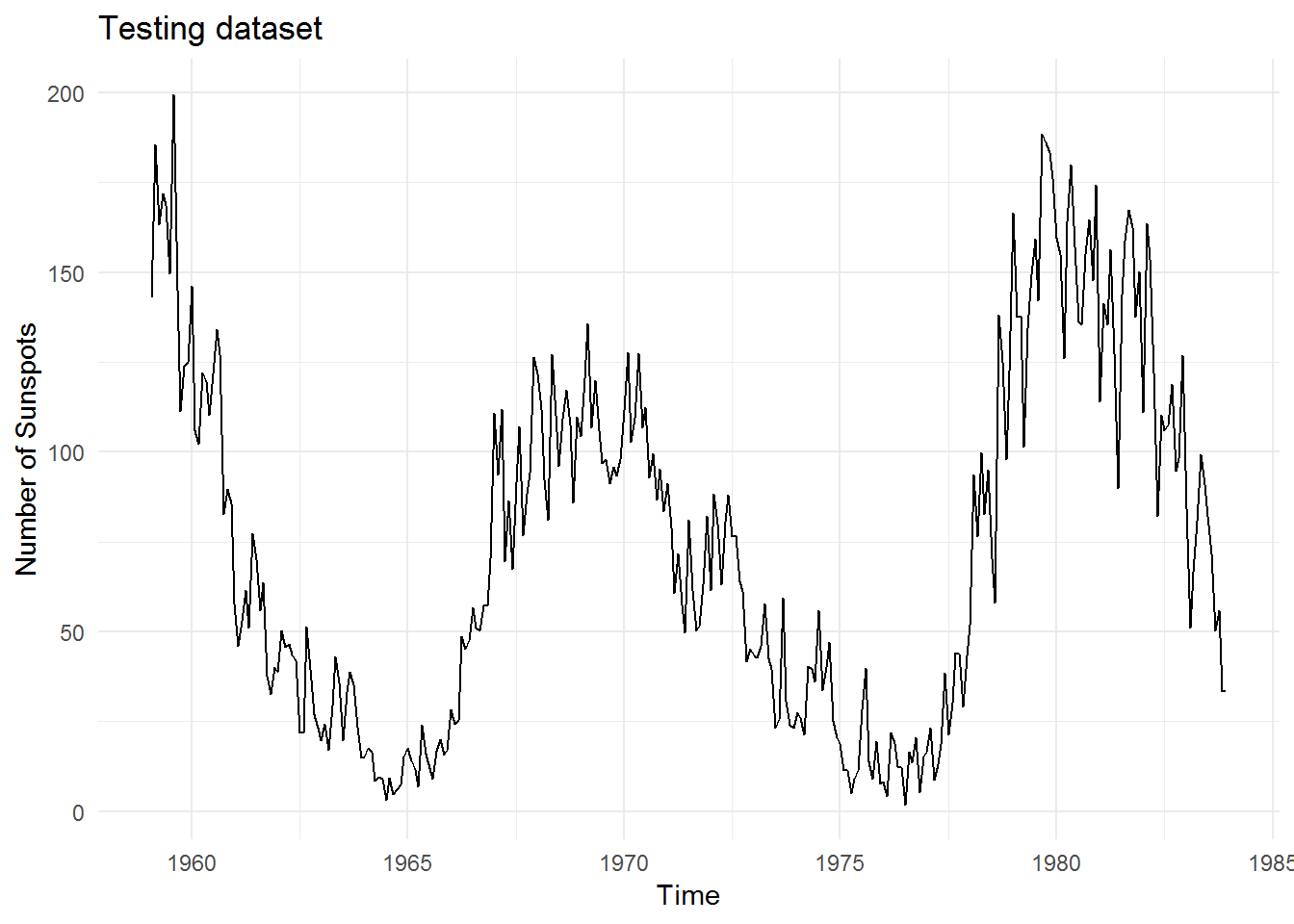
And this is the testing data which we will test our models against:
nnetar
We will use the following code to generate a forecast with nnetar:
# Fitting nnetar model
sun.fit.mlp <- nnetar(sun.train)
sun.fcst.mlp <- forecast(sun.fit.mlp, h = 299)(Note that it only takes 2 lines of code to generate this forecast!)
Here are the model details:
## Series: sun.train
## Model: NNAR(25,1,13)[12]
## Call: nnetar(y = sun.train)
##
## Average of 20 networks, each of which is
## a 25-13-1 network with 352 weights
## options were - linear output units
##
## sigma^2 estimated as 119Keras
Setting up Keras to do a similar forecast is much more involved.
Step 1 - we will need to manually prepare the dataset into a format that Keras can understand. The code is a bunch of scaling, centering and turning the data from a tibble/data.frame to a matrix. I will skip showing that section as I suspect you’ll find it boring and it takes up quite a bit of room.
Step 2 - we can now construct a Keras model:
# Model params
units <- 256
inputs <- 1
# Create model
model.keras <- keras_model_sequential()
model.keras %>%
layer_dense(units = units,
input_shape = c(lookback),
batch_size = inputs,
activation = "relu") %>%
layer_dense(units = units/2,
activation = "relu") %>%
layer_dense(units = units/8,
activation = "relu") %>%
layer_dense(units = 1)
# Compile model
model.keras %>% compile(optimizer = "rmsprop",
loss = "mean_squared_error",
metrics = "accuracy")Step 3 - we can now attempt to train the model:
## Model
## ___________________________________________________________________________
## Layer (type) Output Shape Param #
## ===========================================================================
## dense_1 (Dense) (1, 256) 37120
## ___________________________________________________________________________
## dense_2 (Dense) (1, 128) 32896
## ___________________________________________________________________________
## dense_3 (Dense) (1, 32) 4128
## ___________________________________________________________________________
## dense_4 (Dense) (1, 1) 33
## ===========================================================================
## Total params: 74,177
## Trainable params: 74,177
## Non-trainable params: 0
## ___________________________________________________________________________Step 4 - we can now make predictions from the model:
## Predict based on last observed sunspot number
n <- 299 #number of predictions to make
predictions <- numeric() #vector to hold predictions
# Generate predictions, starting with last observed sunspot number and feeding
# new predictions back into itself
for(i in 1:n){
pred.y <- x[(nrow(x) - inputs + 1):nrow(x), 1:lookback]
dim(pred.y) <- c(inputs, lookback)
# forecast
fcst.y <- model.keras %>% predict(pred.y, batch_size = inputs)
fcst.y <- as_tibble(fcst.y)
names(fcst.y) <- "x"
# Add to previous dataset sun.tibble.rec
sun.tibble.rec <- rbind(sun.tibble.rec, fcst.y)
## Recalc lag matrix
# Setup a lagged matrix (using helper function from nnfor)
sun.tibble.rec.lag <- nnfor::lagmatrix(sun.tibble.rec$x, 0:lookback)
colnames(sun.tibble.rec.lag) <- paste0("x-", 0:lookback)
sun.tibble.rec.lag <- as_tibble(sun.tibble.rec.lag) %>%
filter(!is.na(.[, ncol(.)])) %>%
as.matrix()
# x is input (lag), y is output, multiple inputs
x <- sun.tibble.rec.lag[, 2:(lookback + 1)]
dim(x) <- c(nrow(x), ncol(x))
y <- sun.tibble.rec.lag[, 1]
dim(y) <- length(y)
# Invert recipes
fcst.y <- fcst.y * (range.max.step - range.min.step) + range.min.step
# save prediction
predictions[i] <- fcst.y %>%
InvBoxCox(l)
predictions <- unlist(predictions)
}Results!
And the moment we have been waiting for… which model does a better job at making predictions?