Neural network time series models
November 23, 2017
R modellingI recently became aware of a new neural network time series model in the package nnfor developed by Nikos Kourentzes that really piqued my interest. Let’s put it through some of the test data available in R and compare the two models contained in the nnfor package against the nnetar model contained in Rob Hyndman’s forecast package.
Dataset: AirPassengers
I’ll use the AirPassengers dataset since that’s the dataset that was tested in the nnfor demo, but with some slight modifications. I will establish a training set and a testing set and compare model performance on the testing set only.
Training data:
air.train <- window(AirPassengers, end = 1958)

autoplot(air.train) +
        ylab("Number of Passengers") +
        ggtitle("Training dataset") +
        theme_minimal()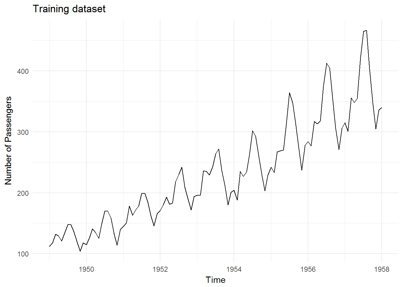
Testing data:
air.test <- window(AirPassengers, start = 1958.001)

autoplot(air.test) +
        ylab("Number of Passengers") +
        ggtitle("Testing dataset") +
        theme_minimal()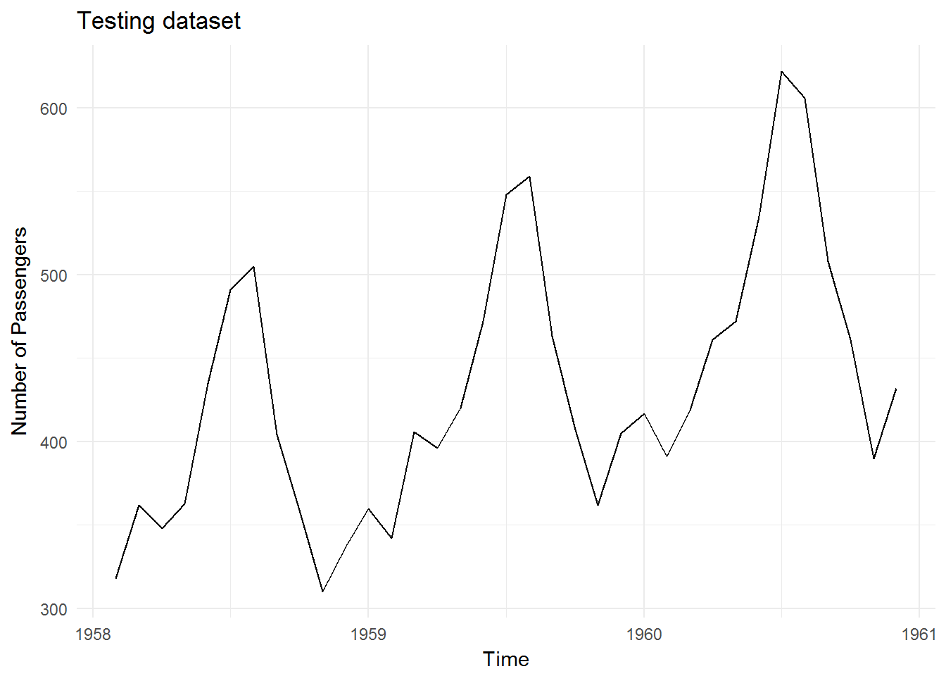
Model prediction comparisons - Defaults
We will run the models with the default/auto parameters first and compare the results.
forecast - Neural Network Autoregression (nnetar)
This neural network model is part of the forecast package. Let’s see how the model performs with default/auto parameters:
# Fitting nnetar model
air.fit.nnetar <- nnetar(air.train)
air.fcst.nnetar <- forecast(air.fit.nnetar, h = 35)
# Visualize model predictions
autoplot(air.test) +
autolayer(air.fcst.nnetar, series = "nnetar Forecast", linetype = "dashed") +
theme_minimal() +
ylab("Number of Passengers")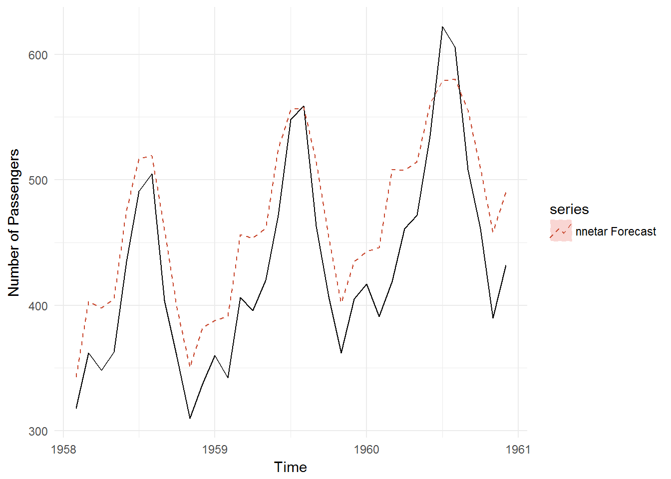
nnfor - Multilayer Perceptrons (MLP)
Moving on to the nnfor package, let’s see how the MLP model performs with default/auto parameters:
# Fitting MLP model
air.fit.mlp <- mlp(air.train)
air.fcst.mlp <- forecast(air.fit.mlp, h = 35)
# Visualize model predictions
autoplot(air.test) +
autolayer(air.fcst.mlp, series = "MLP Forecast", linetype = "dashed") +
theme_minimal() +
ylab("Number of Passengers")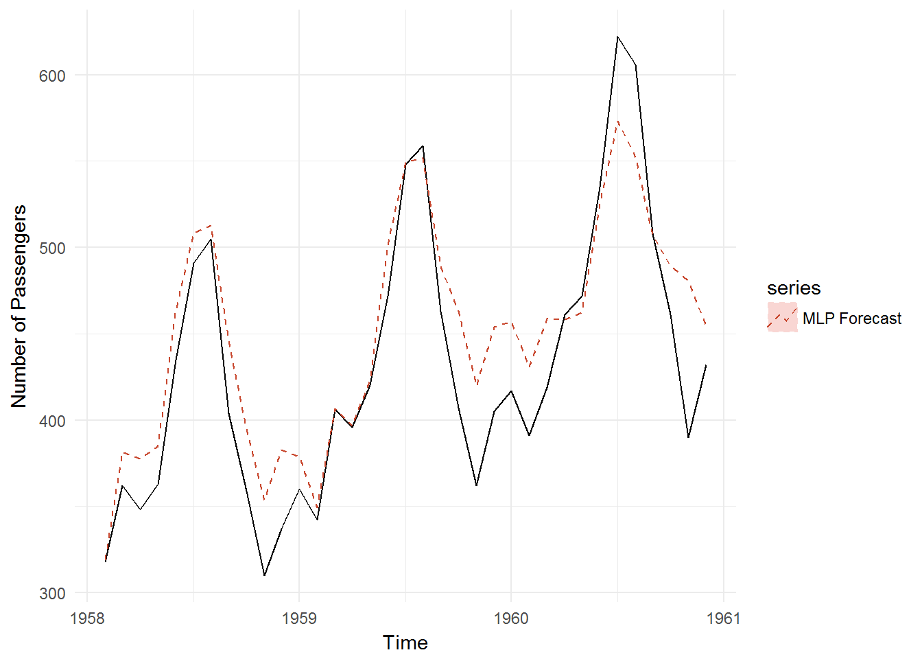
nnfor - Extreme Learning Machine (ELM)
This is the other neural network model available in the nnfor package. Let’s see how the model performs with default/auto parameters:
# Fitting MLP model
air.fit.elm <- elm(air.train)
air.fcst.elm <- forecast(air.fit.elm, h = 35)
# Visualize model predictions
autoplot(air.test) +
autolayer(air.fcst.elm, series = "ELM Forecast", linetype = "dashed") +
theme_minimal() +
ylab("Number of Passengers")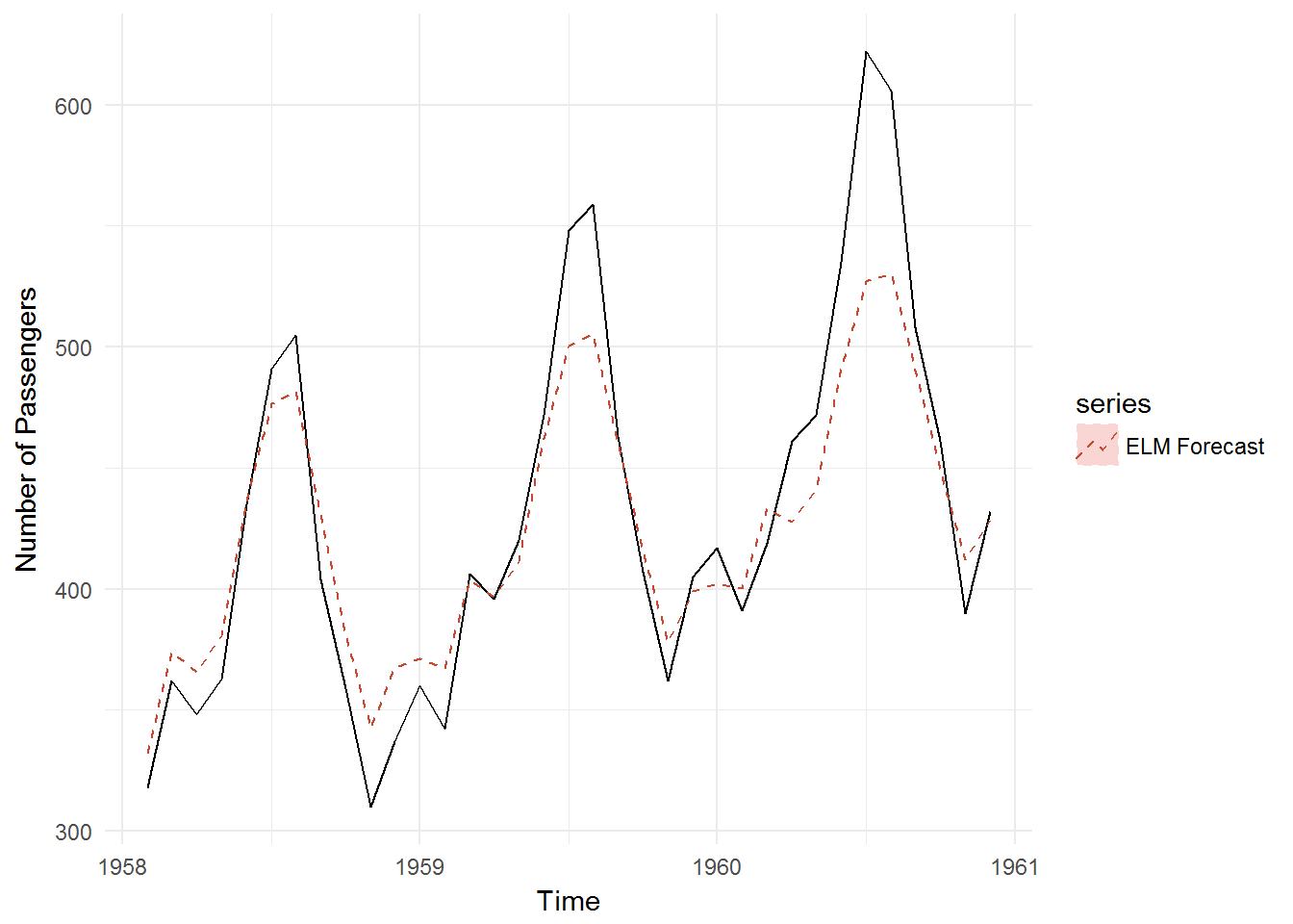
Observations
Visually… I may have to give it to the MLP model here.
Mean absolute error
I’ll use the mean absolute error (MAE) as a more precise measure of model performance. The MAE is the mean difference between each model prediction and the test value, regardless of whether it is over or under the test value.
# Establish tibble to contain predictions
mae <- tibble(Test = air.test,
               nnetar = air.fcst.nnetar$mean,
               MLP = air.fcst.mlp$mean,
               ELM = air.fcst.elm$mean)

# Calculate abs. error
mae$ae.nnetar <- with(mae, abs(nnetar - Test))
mae$ae.MLP <- with(mae, abs(MLP - Test))
mae$ae.ELM <- with(mae, abs(ELM - Test))

# Calculate MAE
mae.score <- apply(mae, 2, mean)[5:7]
names(mae.score) <- c("MAE.nnetar", "MAE.MLP", "MAE.ELM")
mae.score
## MAE.nnetar MAE.MLP MAE.ELM
## 41.47303600 26.76718692 22.26210218And the ELM model wins on default parameters!
Model comparisons - with some tweaks
Let’s play with some of the options in the model functions to see if the results improve. (I’m going to restrict myself to the options in the functions only, without doing any outside transformations, to keep this post relatively light).
I’ll attempt some pre-processing of the data prior to submitting it to the nnetar model and I’ll let the MLP model compute an optimal number of hidden nodes, rather than the default 5. Let’s see if this changes anything.
forecast::nnetar
Starting with forecast::nnetar, we’ll try a BoxCox transformation on the training data first.
# Fitting nnetar model
air.fit.nnetar <- nnetar(air.train, lambda = BoxCox.lambda(air.train))
air.fcst.nnetar <- forecast(air.fit.nnetar, h = 35)
# Visualize model predictions
autoplot(air.test) +
autolayer(air.fcst.nnetar, series = "nnetar w/ BoxCox", linetype = "dashed") +
theme_minimal() +
ylab("Number of Passengers")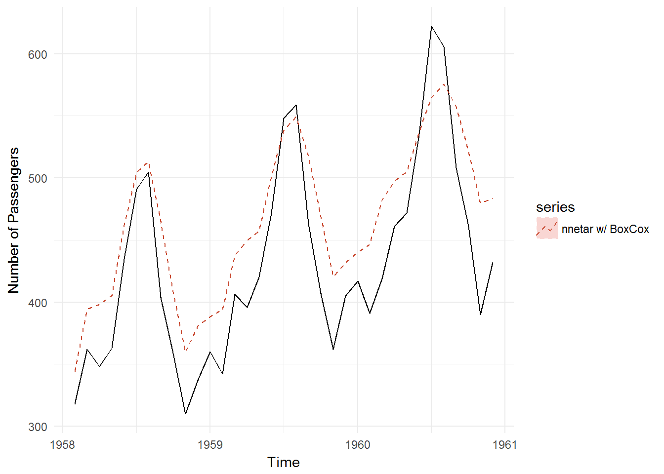
nnfor::mlp
We’ll let MLP compute an optimal number of hidden layers now:
# Fitting MLP model
air.fit.mlp <- mlp(air.train, hd.auto.type = "valid")
air.fcst.mlp <- forecast(air.fit.mlp, h = 35)
# Visualize model predictions
autoplot(air.test) +
autolayer(air.fcst.mlp, series = "MLP w/ opt. hidden nodes", linetype = "dashed") +
theme_minimal() +
ylab("Number of Passengers")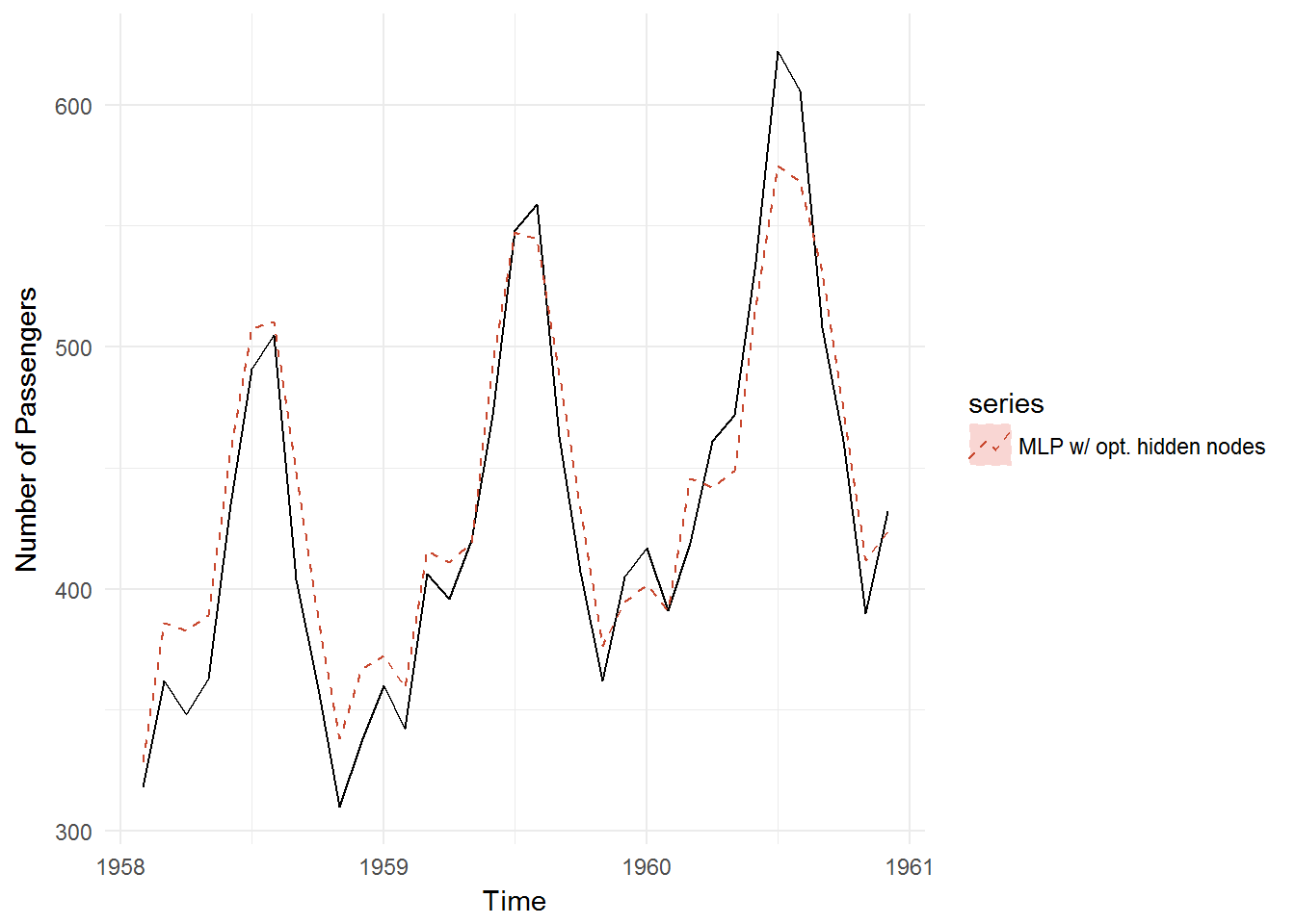
nnfor::elm
I don’t have any quick ideas for tweaking ELM…
Observations
First observation is that the MLP model took a considerable amount of time to compute given that the training dataset had a little over 100 data points. I can see why the default option is 5 nodes rather than a computed number of nodes.
Second observation is that MLP looks really good here.
Mean absolute error
# Establish tibble to contain predictions
mae <- tibble(Test = air.test,
               nnetar = air.fcst.nnetar$mean,
               MLP = air.fcst.mlp$mean,
               ELM = air.fcst.elm$mean)

# Calculate abs. error
mae$ae.nnetar <- with(mae, abs(nnetar - Test))
mae$ae.MLP <- with(mae, abs(MLP - Test))
mae$ae.ELM <- with(mae, abs(ELM - Test))

# Calculate MAE
mae.score <- apply(mae, 2, mean)[5:7]
names(mae.score) <- c("MAE.nnetar", "MAE.MLP", "MAE.ELM")
mae.score
## MAE.nnetar MAE.MLP MAE.ELM
## 40.21540123 19.75997107 22.26210218Looks like nnetar has improved, but MLP has improved more. MLP appears to be pretty promising so far.